TRANSFORM

A series of transformations are applied to the Life Cycle Inventory (LCI) database to align process performance and technology market shares with the outputs from the Integrated Assessment Model (IAM) scenario.

Biomass

Run

from premise import *
import brightway2 as bw

bw.projects.set_current("my_project)

ndb = NewDatabase(
    scenarios=[
            {"model":"remind", "pathway":"SSP2-Base", "year":2028}
        ],
    source_db="ecoinvent 3.7 cutoff",
    source_version="3.7.1",
    key='xxxxxxxxxxxxxxxxxxxxxxxxx'
)
ndb.update("biomass")

Regional biomass markets

premise creates regional markets for biomass which is meant to be used as fuel in biomass-fired powerplants or heat generators. Originally in ecoinvent, the biomass being supplied to biomass-fired powerplants is “purpose grown” biomass that originate forestry activities (called “market for wood chips” in ecoinvent). While this type of biomass is suitable for such purpose, it is considered a co-product of the forestry activity, and bears a share of the environmental burden of the process it originates from (notably the land footprint, emissions, potential use of chemicals, etc.).

However, not all the biomass projected to be used in IAM scenarios is “purpose grown”. In fact, significant shares are expected to originate from forestry residues. In such cases, the environmental burden of the forestry activity is entirely allocated to the determining product (e.g., timber), not to the residue, which comes “free of burden”.

Hence, premise creates average regional markets for biomass, which represents the average shares of “purpose grown” and “residual” biomass being fed to biomass-fired powerplants.

The following market is created for each IAM region:

market name	location
market for biomass, used as fuel	all IAM regions

inside of which, the shares of “purpose grown” and “residual” biomass is represented by the following activities:

name in premise	name in REMIND	name in IMAGE	name in LCI database
biomass - purpose grown	SE|Electricity|Biomass|Energy Crops	Primary Energy|Biomass|Energy Crops	market for wood chips
biomass - residual	SE|Electricity|Biomass|Residues	Primary Energy|Biomass|Residues	supply of forest residue

The sum of those shares equal 1. The activity “supply of forest residue” includes the energy, embodied biogenic CO2, transport and associated emissions to chip the residual biomass and transport it to the powerplant, but no other forestry-related burden is included.

Note

You can check the share of residual biomass used for power generation assumed in your scenarios by generating a scenario summary report.

Note

When running premise with the consequential method, the biomass market is only composed of purpose-grown biomass. This is because the residual biomass cannot be considered a marginal supplier for an increase in demand for biomass.

ndb.generate_scenario_report()

Power generation

Run

from premise import *
import brightway2 as bw

bw.projects.set_current("my_project)

ndb = NewDatabase(
    scenarios=[
            {"model":"remind", "pathway":"SSP2-Base", "year":2028}
        ],
    source_db="ecoinvent 3.7 cutoff",
    source_version="3.7.1",
    key='xxxxxxxxxxxxxxxxxxxxxxxxx'
)
ndb.update("electricity")

The energy conversion efficiency of power plant datasets for specific technologies is adjusted to align with the efficiency changes indicated by the IAM scenario. Two approaches are posisble: * application of a scaling factor to the inputs of the dataset relative to the current efficiency * application of a scaling factor to the inputs of the dataset to match the absolute efficiency given by the IAM scenario

The first approach (default) preserves

Combustion-based powerplants

First, premise adjust the efficiency of coal- and lignite-fired power plants on the basis of the excellent work done by Oberschelp et al. (2019), to update some datasets in ecoinvent, which are, for some of them, several decades old. More specifically, the data provides plant-specific efficiency and emissions factors. We average them by country and fuel type to obtain volume-weighted factors. The efficiency of the following datasets is updated:

• electricity production, hard coal

• electricity production, lignite

• heat and power co-generation, hard coal

• heat and power co-generation, lignite

The data from Oberschelp et al. (2019) also allows us to update emissions of SO2, NOx, CH4, and PMs.

Second, premise iterates through coal, lignite, natural gas, biogas, and wood-fired power plant datasets in the LCI database to calculate their current efficiency (i.e., the ratio between the primary fuel energy entering the process and the output energy produced, which is often 1 kWh). If the IAM scenario anticipates a change in efficiency for these processes, the inputs of the datasets are scaled up or down by the scaling factor to effectively reflect a change in fuel input per kWh produced.

The origin of this scaling factor is the IAM scenario selected.

To calculate the old and new efficiency of the dataset, it is necessary to know the net calorific content of the fuel. The table below shows the Lower Heating Value for the different fuels used in combustion-based power plants.

name of fuel	LHV [MJ/kg, as received]
hard coal	26.7
lignite	11.2
petroleum coke	31.3
wood pellet	16.2
wood chips	18.9
natural gas	45
gas, natural, in ground	45
refinery gas	50.3
propane	46.46
heavy fuel oil	38.5
oil, crude, in ground	38.5
light fuel oil	42.6
biogas	22.73
biomethane	47.5
waste	14
methane, fossil	47.5
methane, biogenic	47.5
methane, synthetic	47.5
diesel	43
gasoline	42.6
petrol, 5% ethanol	41.7
petrol, synthetic, hydrogen	42.6
petrol, synthetic, coal	42.6
diesel, synthetic, hydrogen	43
diesel, synthetic, coal	43
diesel, synthetic, wood	43
diesel, synthetic, wood, with CCS	43
diesel, synthetic, grass	43
diesel, synthetic, grass, with CCS	43
hydrogen, petroleum	120
hydrogen, electrolysis	120
hydrogen, biomass	120
hydrogen, biomass, with CCS	120
hydrogen, coal	120
hydrogen, from natural gas	120
hydrogen, from natural gas, with CCS	120
hydrogen, biogas	120
hydrogen, biogas, with CCS	120
hydrogen	120
biodiesel, oil	38
biodiesel, oil, with CCS	38
bioethanol, wood	26.5
bioethanol, wood, with CCS	26.5
bioethanol, grass	26.5
bioethanol, grass, with CCS	26.5
bioethanol, grain	26.5
bioethanol, grain, with CCS	26.5
bioethanol, sugar	26.5
bioethanol, sugar, with CCS	26.5
ethanol	26.5
methanol, wood	19.9
methanol, grass	19.9
methanol, wood, with CCS	19.9
methanol, grass, with CCS	19.9
liquified petroleum gas, natural	45.5
liquified petroleum gas, synthetic	45.5
uranium, enriched 3.8%, in fuel element for light water reactor	4199040
nuclear fuel element, for boiling water reactor, uo2 3.8%	4147200
nuclear fuel element, for boiling water reactor, uo2 4.0%	4147200
nuclear fuel element, for pressure water reactor, uo2 3.8%	4579200
nuclear fuel element, for pressure water reactor, uo2 4.0%	4579200
nuclear fuel element, for pressure water reactor, uo2 4.2%	4579200
uranium hexafluoride	709166
enriched uranium, 4.2%	4579200
mox fuel element	4579200
heat, from hard coal	1
heat, from lignite	1
heat, from petroleum coke	1
heat, from wood pellet	1
heat, from natural gas, high pressure	1
heat, from natural gas, low pressure	1
heat, from heavy fuel oil	1
heat, from light fuel oil	1
heat, from biogas	1
heat, from waste	1
heat, from methane, fossil	1
heat, from methane, biogenic	1
heat, from diesel	1
heat, from gasoline	1
heat, from bioethanol	1
heat, from biodiesel	1
heat, from liquified petroleum gas, natural	1
heat, from liquified petroleum gas, synthetic	1
bagasse, from sugarcane	15.4
bagasse, from sweet sorghum	13.8
sweet sorghum stem	4.45
cottonseed	21.97
flax husks	21.5
coconut husk	20
sugar beet pulp	5.11
cleft timber	14.46
rape meal	31.1
molasse, from sugar beet	16.65
sugar beet	4.1
barkey grain	19.49
rye grain	12
sugarcane	5.3
palm date	10.8
whey	1.28
straw	15.5
grass	17
manure, liquid	0.875
manure, solid	3.6
kerosene, from petroleum	43
kerosene, synthetic, from electrolysis, energy allocation	43
kerosene, synthetic, from electrolysis, economic allocation	43
kerosene, synthetic, from coal, energy allocation	43
kerosene, synthetic, from coal, economic allocation	43
kerosene, synthetic, from natural gas, energy allocation	43
kerosene, synthetic, from natural gas, economic allocation	43
kerosene, synthetic, from biomethane, energy allocation	43
kerosene, synthetic, from biomethane, economic allocation	43
kerosene, synthetic, from biomass, energy allocation	43
kerosene, synthetic, from biomass, economic allocation	43

Additionally, the biogenic and fossil CO2 emissions of the datasets are also scaled up or down by the same factor, as they are proportional to the amount of fuel used.

Below is an example of a natural gas power plant with a current (2020) conversion efficiency of 77%. If the IAM scenario indicates a scaling factor of 1.03 in 2030, this suggests that the efficiency increases by 3% relative to the current level. As shown in the table below, this would result in a new efficiency of 79%, where all inputs, as well as CO2 emissions outputs, are re-scaled by 1/1.03 (=0.97).

While non-CO2 emissions (e.g., CO) are reduced because of the reduction in fuel consumption, the emission factor per energy unit remains the same (i.e., gCO/MJ natural gas)). It can be re-scaled using the .update(“emissions”) function, which updates emission factors according to GAINS projections.

electricity production, natura gas, conventional	before	after	unit
electricity production	1	1	kWh
natural gas	0.1040	0.1010	m3
water	0.0200	0.0194	m3
powerplant construction	1.00E-08	9.71E-09	unit
CO2, fossil	0.0059	0.0057	kg
CO, fossil	5.87E-06	5.42E-03	kg
fuel-to-electricity efficiency	77%	79%	%

premise has a couple of rules regarding projected scaling factors:

• scaling factors inferior to 1 beyond 2020 are not accepted and are treated as 1.

• scaling factors superior to 1 before 2020 are not accepted and are treated as 1.

• efficiency can only improve over time.

This is to prevent degrading the performance of a technology in the future, or improving its performance in the past, relative to today.

Note

You can check the efficiencies assumed in your scenarios by generating a scenario summary report, or a report of changes. They are automatically generated after each database export, but you can also generate them manually:

ndb.generate_scenario_report()
ndb.generate_change_report()

Photovoltaics panels

Photovoltaic panels are expected to improve over time. The following module efficiencies are considered for the different types of PV panels:

% module efficiency	micro-Si	single-Si	multi-Si	CIGS	CIS	CdTe
2010	10	15.1	14	11	11	10
2020	11.9	17.9	16.8	14	14	16.8
2050	12.5	26.7	24.4	23.4	23.4	21

The sources for these efficiencies are given in the inventory file LCI_PV:

Given a scenario year, premise iterates through the different PV panel installation datasets to update their efficiency accordingly. To do so, the required surface of panel (in m2) per kW of capacity is adjusted down (or up, if the efficiency is lower than current).

To calculate the current efficiency of a PV installation, premise assumes a solar irradiation of 1000 W/m2. Hence, the current efficiency is calculated as:

current_eff [%] = installation_power [W]  / (panel_surface [m2] * 1000 [W/m2])

The scaling factor is calculated as:

scaling_factor = current_eff / new_eff

The required surface of PV panel in the dataset is then adjusted like so:

new_surface = current_surface * (1 / scaling_factor)

For scenario years beyond 2050, 2050 efficiency values are used.

The table below provides such an example where a 450 kWp flat-roof installation sees its current (2020) module efficiency improving from 20% to 26% by 2050. THe are of PV panel (and mounting system) has been multiplied by 1 / (0.26/0.20), all other inputs remaining unchanged.

450kWp flat roof installation	before	after	unit
photovoltaic flat-roof installation, 450 kWp, single-SI, on roof	1	1	unit
inverter production, 500 kW	1.5	1.5	unit
photovoltaic mounting system, …	2300	1731	m2
photovoltaic panel, single-SI	2500	1881	m2
treatment, single-SI PV module	30000	30000	kg
electricity, low voltage	25	25	kWh
module efficiency	20%	26%	%

Markets

premise creates additional datasets that represent the average supply and production pathway for a given commodity for a given scenario, year and region.

Such datasets are called regional markets. Hence, a regional market for high voltage electricity contains the different technologies that supply electricity at high voltage in a given IAM region, in proportion to their respective production volumes.

Regional electricity markets

premise creates high, medium and low-voltage electricity markets for each IAM region. It starts by creating high-voltage markets and define the share of each supplying technology by their respective production volumes in respect to the total volume produced.

High voltage supplying technologies are all technologies besides:

• residential (<=3kWp) photovoltaic power (low voltage)

• waste incineration co-generating powerplants (medium voltage)

Several datasets can qualify for a given technology, in a given IAM region. To define to which extent a given dataset should be supplying in the market, premise uses the current production volume of the dataset.

For example, if coal-fired powerplants are to supply 25% of the high voltage electricity in the IAM region “Europe”, premise fetches the production volumes of all coal-fired powerplants which ecoinvent location is included in the IAM region “Europe” (e.g., DE, PL, LT, etc.), and allocates to each of those a supply share based on their respective production volume in respect to the total production volume of coal-fired powerplants.

For example, the table below shows the contribution of biomass-fired CHP powerplants in the regional high voltage electricity market for IMAGE’s “WEU” region (Western Europe). The biomass CHP technology represents 2.46% of the supply mix. Biomass CHP datasets included in the region “WEU” are given a supply share corresponding to their respective current production volumes.

energy type	Supplier name	Supplier location	Contribution within energy type	Final contribution
Biomass CHP	heat and power co-generation, wood chips	FR	3.80%	0.09%
Biomass CHP	heat and power co-generation, wood chips	AT	2.87%	0.07%
Biomass CHP	heat and power co-generation, wood chips	NO	0.06%	0.00%
Biomass CHP	heat and power co-generation, wood chips	FI	7.65%	0.19%
Biomass CHP	heat and power co-generation, wood chips	SE	9.04%	0.22%
Biomass CHP	heat and power co-generation, wood chips	IT	8.27%	0.20%
Biomass CHP	heat and power co-generation, wood chips	BE	4.59%	0.11%
Biomass CHP	heat and power co-generation, wood chips	DE	12.53%	0.31%
Biomass CHP	heat and power co-generation, wood chips	LU	0.05%	0.00%
Biomass CHP	heat and power co-generation, wood chips	DK	6.60%	0.16%
Biomass CHP	heat and power co-generation, wood chips	GR	0.01%	0.00%
Biomass CHP	heat and power co-generation, wood chips	CH	1.81%	0.04%
Biomass CHP	heat and power co-generation, wood chips	ES	5.10%	0.13%
Biomass CHP	heat and power co-generation, wood chips	PT	1.34%	0.03%
Biomass CHP	heat and power co-generation, wood chips	IE	0.77%	0.02%
Biomass CHP	heat and power co-generation, wood chips	NL	2.32%	0.06%
Biomass CHP	heat and power co-generation, wood chips	GB	33.18%	0.81%
_	_	Sum	100.00%	2.46%

Transformation losses are added to the high-voltage market datasets. Transformation losses are the result of weighting country-specific high voltage losses (provided by ecoinvent) of countries included in the IAM region with their respective current production volumes (also provided by ecoinvent). This is not ideal as it supposes that future country-specific production volumes will remain the same in respect to one another.

Storage

If the IAM scenario requires the use of storage, premise adds a storage dataset to the high voltage market. premise can add two types of storage:

• storage via a large-scale flow battery (electricity supply, high voltage, from vanadium-redox flow battery system)

• storage via the conversion of electricity to hydrogen and subsequent use in a gas turbine (electricity production, from hydrogen-fired one gigawatt gas turbine)

The electricity storage via battery incurs a 33% loss. It is operated by a 8.3 MWh vanadium redox-based flow battery, with a lifetime of 20 years or 8176 cycle-lifes (i.e., 49,000 MWh).

The storage of electricity via hydrogen is done in two steps: first, the electricity is converted to hydrogen via a 1MW PEM electrolyser, with an efficiency of 62%. The hydrogen is then stored in a geological cavity and used in a gas turbine, with an efficiency of 51%. Accounting for leakages and losses, the overall efficiency of the process is about 37% (i.e., 2.7 kWh necessary to deliver 1 kWh to the grid).

The efficiency of the H2-fed gas turbine is based on the parameters of Ozawa et al. (2019).

The workflow is not too different from that of high voltage markets. There are however only two possible providers of electricity in medium voltage markets: the high voltage market, as well as waste incineration powerplants.

High-to-medium transformation losses are added as an input of the medium voltage market to itself. Distribution losses are modelled the same way as for high voltage markets and are added to the input from high voltage market.

Low voltage regional markets receive an input from the medium voltage market, as well as from residential photovoltaic power.

Medium-to-low transformation losses are added as an input from the low voltage market to itself. Distribution losses are modelled the same way as for high and medium voltage markets, and are added to the input from the medium voltage market.

The table below shows the example of a low voltage market for the IAM IMAGE regional “WEU”.

supplier	amount	unit	location	description
market group for electricity, medium voltage	1.023880481	kilowatt hour	WEU	input from medium voltage + distribution losses
market group for electricity, low voltage	0.025538286	kilowatt hour	WEU	transformation losses (2.55%)
electricity production, photovoltaic, residential	0.00035691	kilowatt hour	DE
electricity production, photovoltaic, residential	0.000143875	kilowatt hour	IT
electricity production, photovoltaic, residential	9.38E-05	kilowatt hour	ES
electricity production, photovoltaic, residential	9.03E-05	kilowatt hour	GB
electricity production, photovoltaic, residential	7.82E-05	kilowatt hour	FR
electricity production, photovoltaic, residential	6.80E-05	kilowatt hour	NL
electricity production, photovoltaic, residential	3.76E-05	kilowatt hour	BE
electricity production, photovoltaic, residential	2.16E-05	kilowatt hour	GR
electricity production, photovoltaic, residential	2.08E-05	kilowatt hour	CH
electricity production, photovoltaic, residential	1.48E-05	kilowatt hour	AT
electricity production, photovoltaic, residential	9.44E-06	kilowatt hour	SE
electricity production, photovoltaic, residential	8.66E-06	kilowatt hour	DK
electricity production, photovoltaic, residential	6.83E-06	kilowatt hour	PT
electricity production, photovoltaic, residential	2.60E-06	kilowatt hour	FI
electricity production, photovoltaic, residential	1.30E-06	kilowatt hour	LU
electricity production, photovoltaic, residential	1.01E-06	kilowatt hour	NO
electricity production, photovoltaic, residential	2.40E-07	kilowatt hour	IE
distribution network construction, electricity, low voltage	8.74E-08	kilometer	RoW
market for sulfur hexafluoride, liquid	2.99E-09	kilogram	RoW
sulfur hexafluoride	2.99E-09	kilogram		transformer emissions

Note

You can check the electricity supply mixes assumed in your scenarios by generating a scenario summary report.

ndb.generate_scenario_report()

Long-term regional electricity markets

Long-term (i.e., 20, 40 and 60 years) regional markets are created for modelling the lifetime-weighted burden associated to electricity supply for systems that have a long lifetime (e.g., battery electric vehicles, buildings).

These long-term markets contain a period-weighted electricity supply mix. For example, if the scenario year is 2030 and the period considered is 20 years, the supply mix represents the supply mixes between 2030 and 2050, with an equal weight given to each year.

The rest of the modelling is similar to that of regular regional electricity markets described above.

Market datasets originally present in the ecoinvent LCI database are cleared from any inputs. Instead, an input from the newly created regional market is added, depending on the location of the dataset.

The table below shows the example of the low voltage electricity market for Great Britain, which now only includes an input from the “WEU” regional market, which “includes” it in terms of geography.

Output	_	_	_
producer	amount	unit	location
market for electricity, low voltage	1.00E+00	kilowatt hour	GB
Input	_	_	_
supplier	amount	unit	location
market group for electricity, low voltage	1.00E+00	kilowatt hour	WEU

Once the new markets are created, premise re-links all electricity-consuming activities to the new regional markets. The regional market it re-links to depends on the location of the consumer.

Cement production

The modelling of future improvements in the cement sector is relatively simple at the moment, and does not involve the emergence of new technologies (e.g., electric kilns).

Run

from premise import *
import brightway2 as bw

bw.projects.set_current("my_project)

ndb = NewDatabase(
    scenarios=[
            {"model":"remind", "pathway":"SSP2-Base", "year":2028}
        ],
    source_db="ecoinvent 3.7 cutoff",
    source_version="3.7.1",
    key='xxxxxxxxxxxxxxxxxxxxxxxxx'
)
ndb.update("cement")

premise duplicates clinker production datasets in ecoinvent (called “clinker production”) so as to create a proxy dataset for each IAM region. The location of the proxy datasets used for a given IAM region is a location included in the IAM region. If no valid dataset is found, premise resorts to using a rest-of-the-world (RoW) dataset to represent the IAM region.

premise changes the location of these duplicated datasets and fill in different fields, such as that of production volume.

premise then adjusts the thermal efficiency of the process. It does so by calculating the technology-weighted energy requirements per ton of clinker. Based on GNR/IEA roadmap data, premise uses:

• the share of kiln technology for a given region today (2020):

  • wet,

  • dry,

  • dry with pre-heater,

  • and dry with pre-heater and pre-calciner

• the energy requirement for each of these technologies today (2020).

Once the energy required per ton clinker today (2020) is known, it is multiplied by a scaling factor that represents a change in efficiency between today and the scenario year.

Note

You can check the efficiency gains assumed relative to 2020 in your scenarios by generating a scenario summary report.

ndb.generate_scenario_report()

Note

premise enforces a lower limit on the fuel consumption per ton of clinker. This limit is set to 2.8 GJ/t clinker and corresponds to the minimum theoretical fuel consumption with an moisture content of the raw materials, as considered in the 2018 IEA cement roadmap report. Hence, regardless of the scaling factor, the fuel consumption per ton of clinker will never be less than 2.8 GJ/t.

Once the new energy input is determined, premise scales down the fuel, and the fossil and biogenic CO2 emissions accordingly, based on the Lower Heating Value and CO2 emission factors for these fuels.

Note that the change in CO2 emissions only concerns the share that originates from the combustion of fuels. It does not concern the calcination emissions due to the production of calcium oxide (CaO) from calcium carbonate (CaCO3), which is set at a fix emission rate of 525 kg CO2/t clinker.

If the IAM scenario indicates that a share of the CO2 emissions for the cement sector in a given region and year is sequestered and stored, premise adds CCS to the corresponding clinker production dataset.

The CCS dataset used to that effect is from Meunier et al., 2020. The dataset described the capture of CO2 from a cement plant. To that dataset, premise adds another dataset that models the storage of the CO2 underground, from Volkart et al, 2013.

Besides electricity, the CCS process requires heat, water and others inputs to regenerate the amine-based sorbent. We use two data points to approximate the heat requirement: 3.66 MJ/kg CO2 captured in 2020, and 2.6 MJ/kg in 2050. The first number is from Meunier et al., 2020, while the second number is described as the best-performing pilot project today, according to the 2022 review of pilot projects by the Global CCS Institute. It is further assumed that the heat requirement is fulfilled to an extent of 15% by the recovery of excess heat, as mentioned in the 2018 IEA cement roadmap report.

Note

You can check the the carbon capture rate for cement production assumed in your scenarios by generating a scenario summary report.

ndb.generate_scenario_report()

Run

from premise import *
import brightway2 as bw

bw.projects.set_current("my_project)

ndb = NewDatabase(
    scenarios=[
            {"model":"remind", "pathway":"SSP2-Base", "year":2028}
        ],
    source_db="ecoinvent 3.7 cutoff",
    source_version="3.7.1",
    key='xxxxxxxxxxxxxxxxxxxxxxxxx'
)
ndb.update("cement")

When clinker production datasets are created for each IAM region, premise duplicates cement production datasets for each IAM region as well. These cement production datasets link the newly created clinker production dataset, corresponding to their IAM region.

premise used to modify the composition of cement markets to reflect a lower clinker content over time, based on external projections. This is no longer performed, as it is not an assumption stemming from the IAM model, but rather a projection of the cement industry.

Market datasets originally present in the ecoinvent LCI database are cleared from any inputs. Instead, an input from the newly created regional market is added, depending on the location of the dataset.

The table below shows the example of the clinker market for South Africa, which now only includes an input from the “SAF” regional market, which “includes” it in terms of geography.

Output	_	_	_
producer	amount	unit	location
market for clinker	1.00E+00	kilogram	ZA
Input	_	_	_
supplier	amount	unit	location
market for clinker	1.00E+00	kilogram	*SAF

Once cement production and market datasets are created, premise re-links cement-consuming activities to the new regional markets for cement. The regional market it re-links to depends on the location of the consumer.

Steel production

Run

from premise import *
import brightway2 as bw

bw.projects.set_current("my_project)

ndb = NewDatabase(
    scenarios=[
            {"model":"remind", "pathway":"SSP2-Base", "year":2028}
        ],
    source_db="ecoinvent 3.7 cutoff",
    source_version="3.7.1",
    key='xxxxxxxxxxxxxxxxxxxxxxxxx'
)
ndb.update("steel")"

The modelling of future improvements in the steel sector is relatively simple at the moment, and does not involve the emergence of new technologies (e.g., hydrogen-based DRI, electro-winning).

premise duplicates steel production datasets in ecoinvent for the production of primary and secondary steel (called respectively “steel production, converter” and “steel production, electric”) so as to create a proxy dataset for each IAM region.

The location of the proxy datasets used for a given IAM region is a location included in the IAM region. If no valid dataset is found, premise resorts to using a rest-of-the-world (RoW) dataset to represent the IAM region.

premise changes the location of these duplicated datasets and fill in different fields, such as that of production volume.

Regarding primary steel production (using BO-BOF), premise adjusts the inputs of fuels found in:

• the pig iron production datasets,

• the steel production datasets,

assuming an integrated steel mill unit, by multiplying these fuel inputs by a scaling factor provided by the IAM scenario.

Typical fuel inputs for these process are natural gas, coal, coal-based coke. Emissions of (fossil) CO2 are scaled accordingly.

Regarding the production of secondary steel (using EAF), premise adjusts the input of electricity based on the scaling factor provided by the IAM scenario.

Note

You can check the efficiency gains assumed relative to 2020 for steel production in your scenarios by generating a scenario summary report.

ndb.generate_scenario_report()

Warning

If your system of interest relies heavily on the provision of steel, you should probably consider modelling steel production based on primary data. ecoinvent datasets for steel production rely on a few data points, which are then further process transformed by premise. Therefore, there is a large modelling uncertainty.

If the IAM scenario indicates that a share of the CO2 emissions from the steel sector in a given region and year is sequestered and stored, premise adds a corresponding input from a CCS dataset. The datatset used to that effect is from Meunier et al., 2020. The dataset described the capture of CO2 from a cement plant, not a steel mill, but it is assumed to be an acceptable approximation since the CO2 concentration in the flue gases should not be significantly different.

To that dataset, premise adds another dataset that models the storage of the CO2 underground, from Volkart et al, 2013.

Besides electricity, the CCS process requires heat, water and others inputs to regenerate the amine-based sorbent. We use two data points to approximate the heat requirement: 3.66 MJ/kg CO2 captured in 2020, and 2.6 MJ/kg in 2050. The first number is from Meunier et al., 2020, while the second number is described as the best-performing pilot project today, according to the 2022 review of pilot projects by the Global CCS Institute. It is further assumed that the heat requirement is fulfilled to an extent of 15% by the recovery of excess heat, as mentioned in the 2018 IEA cement roadmap report, which is assumed to be also valid in the case of a steel mill.

premise create a dataset “market for steel, low-alloyed” for each IAM region. Within each dataset, the supply shares of primary and secondary steel are adjusted to reflect the projections from the IAM scenario, for a given region and year, based on the variables below.

name in premise	name in REMIND	name in IMAGE	name in LCI database
steel - primary	Production|Industry|Steel|Primary	Production|Steel|Primary	steel production, converter
steel - secondary	Production|Industry|Steel|Secondary	Production|Steel|Secondary	steel production, electric

The table below shows an example of the market for India, where 66% of the steel comes from an oxygen converter process (primary steel), while 34% comes from an electric arc furnace process (secondary steel).

Output	_	_	_
producer	amount	unit	location
market for steel, low-alloyed	1	kilogram	IND
Input
supplier	amount	unit	location
market group for transport, freight, inland waterways, barge	0.5	ton kilometer	GLO
market group for transport, freight train	0.35	ton kilometer	GLO
market for transport, freight, sea, bulk carrier for dry goods	0.38	ton kilometer	GLO
transport, freight, lorry, unspecified, regional delivery	0.12	ton kilometer	IND
steel production, converter, low-alloyed	0.66	kilogram	IND
steel production, electric, low-alloyed	0.34	kilogram	IND

Market datasets originally present in the ecoinvent LCI database are cleared from any inputs. Instead, an input from the newly created regional market is added, depending on the location of the dataset.

The table below shows the example of the clinker market for South Africa, which now only includes an input from the “SAF” regional market, which “includes” it in terms of geography.

Output	_	_	_
producer	amount	unit	location
market for clinker	1.00E+00	kilogram	ZA
Input	_	_	_
supplier	amount	unit	location
market for clinker	1.00E+00	kilogram	SAF

Once steel production and market datasets are created, premise re-links steel-consuming activities to the new regional markets for steel. The regional market it re-links to depends on the location of the consumer.

Transport

Run

from premise import *
import brightway2 as bw

bw.projects.set_current("my_project)

ndb = NewDatabase(
    scenarios=[
            {"model":"remind", "pathway":"SSP2-Base", "year":2028}
        ],
    source_db="ecoinvent 3.7 cutoff",
    source_version="3.7.1",
    key='xxxxxxxxxxxxxxxxxxxxxxxxx'
)
ndb.update("two_wheelers")
ndb.update("cars")
ndb.update("trucks")
ndb.update("buses")

premise imports inventories for transport activity operated by:

• two-wheelers

• passenger cars

• medium and heavy duty trucks

• buses

These inventories are available for the construction year of 2000 to 2050, by steps of 5 years, but premise only imports vehicles with a construction year inferior or equal to the scenario year (vehicle from 2050 will not be imported in a database for the scenario year of 2030, but vehicles from 2020 will, as they are necessary to build the fleet average vehicles).

The following size classes of medium and heavy duty trucks are imported:

• 3.5t

• 7.5t

• 18t

• 26t

• 40t

These weights refer to the vehicle gross mass (the maximum weight the vehicle is allowed to reach, fully loaded).

Each truck is available for a variety of powertrain types:

• fuel cell electric

• battery electric

• diesel hybrid

• plugin diesel hybrid

• diesel

• compressed gas

but also for different driving cycles, to which a range autonomy of the vehicle is associated:

• urban delivery (required range autonomy of 150 km)

• regional delivery (required range autonomy of 400 km)

• long haul (required range autonomy of 800 km)

Those are driving cycles developed for the software VECTO, which have become standard in measuring the CO2 emissions of trucks.

The truck vehicle model is from Sacchi et al, 2021.

Note

Not all powertrain types are available for regional and long haul driving cycles. This is specifically the case for battery electric trucks, for which the mass and size prevent them from completing the cycle, or surpasses the vehicle gross weight.

Warning

A consequence of replacing original truck datasets with those provided by premise may be a steep increase in CO2-eq. emissions, especially if the urban driving cycle is chosen. Overall, considering and size classes, diesel truck datasets from ecoinvent have lower fuel consumption and exhaust emissions.

Fleet average trucks

REMIND and IMAGE provide fleet composition data, per scenario, region and year.

The fleet data is expressed in “vehicle-kilometer” performed by each type of vehicle, in a given region and year.

premise uses the following loads to translate the transport demand from “vehicle-kilometers” to “ton-kilometers”, derived from TRACCS:

load [tons]	urban delivery	regional delivery	long haul
3.5t	0.26	0.26	0.8
7.5t	0.52	0.52	1.6
18t	1.35	1.35	4.1
26t	2.05	2.05	6.2
32t	6.1	6.1	9.1
40t	6.1	6.1	9.1

Note

Loads from the TRACCS survey data are representative for EU-28 conditions. premise applies these loads to all IAM regions. Hence, there might be some inconsistency at this level. Also, these loads are much lower than those assumed in original ecoinvent truck datasets.

premise uses the fleet data to produce fleet average trucks for each IAM region, and more specifically:

• a fleet average truck, all powertrains and size classes considered

• a fleet average truck, all powertrains considered, for a given size class

They appear in the LCI database as the following:

truck transport dataset name	description
transport, freight, lorry, 3.5t gross weight, unspecified powertrain, long haul	fleet average, for 3.5t size class, long haul cycle
transport, freight, lorry, 3.5t gross weight, unspecified powertrain, regional delivery	fleet average, for 3.5t size class, regional delivery cycle
transport, freight, lorry, 3.5t gross weight, unspecified powertrain, urban delivery	fleet average, for 3.5t size class, urban delivery cycle
transport, freight, lorry, 7.5t gross weight, unspecified powertrain, long haul	fleet average, for 7.5t size class, long haul cycle
transport, freight, lorry, 7.5t gross weight, unspecified powertrain, regional delivery	fleet average, for 7.5t size class, regional delivery cycle
transport, freight, lorry, 7.5t gross weight, unspecified powertrain, urban delivery	fleet average, for 7.5t size class, urban delivery cycle
transport, freight, lorry, 18t gross weight, unspecified powertrain, long haul	fleet average, for 18t size class, long haul cycle
transport, freight, lorry, 18t gross weight, unspecified powertrain, regional delivery	fleet average, for 18t size class, regional delivery cycle
transport, freight, lorry, 18t gross weight, unspecified powertrain, urban delivery	fleet average, for 18t size class, urban delivery cycle
transport, freight, lorry, 26t gross weight, unspecified powertrain, long haul	fleet average, for 26t size class, long haul cycle
transport, freight, lorry, 26t gross weight, unspecified powertrain, regional delivery	fleet average, for 26t size class, regional delivery cycle
transport, freight, lorry, 26t gross weight, unspecified powertrain, urban delivery	fleet average, for 26t size class, urban delivery cycle
transport, freight, lorry, 40t gross weight, unspecified powertrain, long haul	fleet average, for 26t size class, long haul cycle
transport, freight, lorry, 40t gross weight, unspecified powertrain, regional delivery	fleet average, for 26t size class, regional delivery cycle
transport, freight, lorry, 40t gross weight, unspecified powertrain, urban delivery	fleet average, for 26t size class, urban delivery cycle
transport, freight, lorry, unspecified, long haul	fleet average, all powertrain types, all size classes
transport, freight, lorry, unspecified, regional delivery	fleet average, all powertrain types, all size classes
transport, freight, lorry, unspecified, urban delivery	fleet average, all powertrain types, all size classes

Relinking

Regarding trucks, premise re-links truck transport-consuming activities to the newly created fleet average truck datasets.

The following table shows the correspondence between the original truck transport datasets and the new ones replacing them:

Original dataset	Replaced by (REMIND)	Replaced by (IMAGE)
transport, freight, lorry, unspecified	transport, freight, lorry, unspecified	transport, freight, lorry, unspecified
transport, freight, lorry 16-32 metric ton	transport, freight, lorry, 26t gross weight, unspecified powertrain	transport, freight, lorry, 26t gross weight, unspecified powertrain
transport, freight, lorry 28 metric ton, fatty acid methyl ester 100%	transport, freight, lorry, 26t gross weight, unspecified powertrain	transport, freight, lorry, 26t gross weight, unspecified powertrain
transport, freight, lorry 3.5-7.5 metric ton	transport, freight, lorry, 3.5t gross weight, unspecified powertrain	transport, freight, lorry, 26t gross weight, unspecified powertrain
transport, freight, lorry 7.5-16 metric ton	transport, freight, lorry, 7.5t gross weight, unspecified powertrain	transport, freight, lorry, 26t gross weight, unspecified powertrain
transport, freight, lorry >32 metric ton	transport, freight, lorry, 40t gross weight, unspecified powertrain	transport, freight, lorry, 40t gross weight, unspecified powertrain
transport, freight, lorry with reefer, cooling	transport, freight, lorry, unspecified	transport, freight, lorry, unspecified
transport, freight, lorry with reefer, freezing	transport, freight, lorry, unspecified	transport, freight, lorry, unspecified
transport, freight, lorry with refrigeration machine, 3.5-7.5 ton	transport, freight, lorry, 3.5t gross weight, unspecified powertrain	transport, freight, lorry, 26t gross weight, unspecified powertrain
transport, freight, lorry with refrigeration machine, 7.5-16 ton	transport, freight, lorry, 7.5t gross weight, unspecified powertrain	transport, freight, lorry, 26t gross weight, unspecified powertrain
transport, freight, lorry with refrigeration machine, cooling	transport, freight, lorry, unspecified	transport, freight, lorry, unspecified
transport, freight, lorry with refrigeration machine, freezing	transport, freight, lorry, unspecified	transport, freight, lorry, unspecified

Note that IMAGE fleet data only uses 26t and 40t trucks.

Additionally, premise iterates through each truck transport-consuming activities to calculate the driving distance required. When the reference unit of the dataset is 1 kilogram, the distance driven by truck can easily be inferred. Indeed, for example, 0.56 tkm of truck transport for 1 kg of flour indicates that the flour has been transported over 560 km.

On this basis, premise chooses one of the following driving cycles:

• regional delivery, if the distance is inferior or equal to 450 km

• long haul, if the distance is superior to 450 km

Hence, in the following dataset for “market for steel, low-alloyed” for the IAM region of India, premise chose the regional delivery driving cycle since the kilogram of steel has been transported on average over 120 km by truck. The truck used to transport that kilogram of steel is a fleet average vehicle built upon the REMIND fleet data for the region of India.

Output	_	_	_
producer	amount	unit	location
market for steel, low-alloyed	1	kilogram	IND
Input
supplier	amount	unit	location
market group for transport, freight, inland waterways, barge	0.5	ton kilometer	GLO
market group for transport, freight train	0.35	ton kilometer	GLO
market for transport, freight, sea, bulk carrier for dry goods	0.38	ton kilometer	GLO
transport, freight, lorry, unspecified, regional delivery	0.12	ton kilometer	IND
steel production, converter, low-alloyed	0.66	kilogram	IND
steel production, electric, low-alloyed	0.34	kilogram	IND

Direct Air Capture

Run

from premise import *
import brightway2 as bw

bw.projects.set_current("my_project)

ndb = NewDatabase(
    scenarios=[
            {"model":"remind", "pathway":"SSP2-Base", "year":2028}
        ],
    source_db="ecoinvent 3.7 cutoff",
    source_version="3.7.1",
    key='xxxxxxxxxxxxxxxxxxxxxxxxx'
)
ndb.update("dac")

premise creates different region-specific Direct Air Capture (DAC) datasets, based on the inventories from Qiu et al., 2022.

If provided by the IAM scenario, premise scales the inputs of electricity and heat of the DAC datasets to reflect changes in efficiency.

Fuels

Run

from premise import *
import brightway2 as bw

bw.projects.set_current("my_project)

ndb = NewDatabase(
    scenarios=[
            {"model":"remind", "pathway":"SSP2-Base", "year":2028}
        ],
    source_db="ecoinvent 3.7 cutoff",
    source_version="3.7.1",
    key='xxxxxxxxxxxxxxxxxxxxxxxxx'
)
ndb.update("fuels")

premise create different region-specific fuel supply chains and fuel markets, based on data from the IAM scenario.

The biomass-to-fuel efficiency ratio of bioethanol and biodiesel production datasets is adjusted according to the IAM scenario projections.

Inputs to the biofuel production datasets are multiplied by a scaling factor that represents the change in efficiency relative to today (2020).

Several pathways for hydrogen production are modeled in premise:

• electrolysis

• steam methane reforming of natural gas

• steam methane reforming of biomethane

• gasification of coal

• gasification of woody biomass

The last four pathways are modeled with and without CCS.

Inventories for these pathways are available under:

• premise/data/additional_inventories/lci-hydrogen-electrolysis.xlsx

• premise/data/additional_inventories/lci-smr-atr-natgas.xlsx

• premise/data/additional_inventories/lci-smr-atr-biogas.xlsx

• premise/data/additional_inventories/lci-hydrogen-coal-gasification.xlsx

• premise/data/additional_inventories/lci-hydrogen-wood-gasification.xlsx

In case the IAM variable that relates to a given hydrogen pathway’s efficiency is not available, the process’ efficiency is not modified, with the exception of electrolysis, which is modified regardless.

A scaling factor is calculated for each pathway, which is the ratio between the IAM variable value for the year in question and the current efficiency value (i.e., in 2020). premise uses this scaling factor to adjust the amount of feedstock input to produce 1 kg of hydrogen (e.g., m3 of natural gas per kg hydrogen).

If the IAM variable that relates to the efficiency of the electrolysis hydrogen process is not available, premise adjusts the amount of electricity needed to produce 1 kg of hydrogen by electrolysis, on the basis of the following requirements, which are sourced from Bauer et al, 2022:

kWh/kg H2, 25 bar	2010	2020	2050
electricity	58	55	44

When building a database using IMAGE, land use and land use change emissions are available. Upon the import of crops farming datasets, premise adjusts the land occupation as well as CO2 emissions associated to land use and land use change, respectively.

Output	_	_	_
producer	amount	unit	location
Farming and supply of corn	1	kilogram	CEU
Input
supplier	amount	unit	location
market for diesel, burned in agricultural machinery	0.142	megajoule	GLO
petrol, unleaded, burned in machinery	0.042	megajoule	GLO
market for natural gas, burned in gas motor, for storage	0.091	megajoule	GLO
market group for electricity, low voltage	0.004	kilowatt hour	CEU
Energy, gross calorific value, in biomass	15.910	megajoule	_
Occupation, annual crop	1.584	square meter-year	_
Carbon dioxide, in air	1.476	kilogram	_
Carbon dioxide, from soil or biomass stock	1.140	kilogram	_

The land use value is given from the IAM scenario in Ha/GJ of primary crop energy. Hence, the land occupation per kg of crop farmed is calculated as:

land_use = land_use [Ha/GJ] * 10000 [m2/Ha] / 1000 [MJ/GJ] * LHV [MJ/kg]

Regarding land use change CO2 emissions, the principle is similar. The variable is expressed in kg CO2/GJ of primary crop energy. Hence, the land use change CO2 emissions per kg of crop farmed are calculated as:

land_use_co2 = land_use_co2 [kg CO2/GJ] / 1000 [MJ/GJ] * LHV [MJ/kg]

premise builds several supply chains for synthetic fuels, for each IAM region. THe reason for this is that synthetic fuels can be produced from a variety of hydrogen and CO2 sources. Additionally, hydrogen can be supplied by different means of transport, and in different states.

premise starts by building different supply chains for hydrogen by varying:

• the transport mode: truck, hydrogen pipeline, re-assigned CNG pipeline, ship,

• the distance: 500 km, 2000 km

• the state of the hydrogen: gaseous, liquid, liquid organic compound,

• the hydrogen production route: electrolysis, SMR, biomass gasifier (coal, woody biomass)

Hence, for each IAM region, the following supply chains for hydrogen are built:

• hydrogen supply, from electrolysis, by ship, as liquid, over 2000 km

• hydrogen supply, from gasification of biomass by heatpipe reformer, by H2 pipeline, as gaseous, over 500 km

• hydrogen supply, from ATR of from natural gas, by truck, as gaseous, over 500 km

• hydrogen supply, from gasification of biomass by heatpipe reformer, by truck, as liquid organic compound, over 500 km

• hydrogen supply, from SMR of from natural gas, with CCS, by truck, as liquid organic compound, over 500 km

• hydrogen supply, from SMR of from natural gas, with CCS, by ship, as liquid, over 2000 km

• hydrogen supply, from coal gasification, by CNG pipeline, as gaseous, over 500 km

• hydrogen supply, from SMR of from natural gas, by ship, as liquid, over 2000 km

• hydrogen supply, from coal gasification, by truck, as liquid, over 500 km

• hydrogen supply, from gasification of biomass by heatpipe reformer, by truck, as liquid, over 500 km

• hydrogen supply, from ATR of from natural gas, with CCS, by truck, as liquid organic compound, over 500 km

• hydrogen supply, from SMR of from natural gas, with CCS, by truck, as liquid, over 500 km

• hydrogen supply, from electrolysis, by truck, as liquid organic compound, over 500 km

• hydrogen supply, from gasification of biomass, by truck, as liquid organic compound, over 500 km

• hydrogen supply, from SMR of from natural gas, with CCS, by truck, as gaseous, over 500 km

• hydrogen supply, from SMR of biogas, with CCS, by CNG pipeline, as gaseous, over 500 km

• hydrogen supply, from SMR of from natural gas, by truck, as gaseous, over 500 km

• hydrogen supply, from SMR of from natural gas, by H2 pipeline, as gaseous, over 500 km

• hydrogen supply, from gasification of biomass, with CCS, by truck, as liquid organic compound, over 500 km

• hydrogen supply, from gasification of biomass, by ship, as liquid, over 2000 km

Each supply route is associated with specific losses. Losses for the transport of H2 by truck and hydrogen pipelines, and losses at the regional storage storage (salt cavern) are from Wulf et al, 2018. Boil-off loss values during shipping are from Hank et al, 2020. Losses when transporting H2 via re-assigned CNG pipelines are from Cerniauskas et al, 2020. Losses along the pipeline are from Schori et al, 2012., but to be considered conservative, as those are initially for natural gas (and hydrogen has a higher potential for leaking).

_	_	truck	ship	H2 pipeline	CNG pipeline	reference flow
gaseous	compression	0.5%		0.5%	0.5%	per kg H2
_	storage buffer			2.3%	2.3%	per kg H2
_	storage leak			1.0%	1.0%	per kg H2
_	pipeline leak			0.004%	0.004%	per kg H2, per km
_	purification				7.0%	per kg H2
liquid	liquefaction	1.3%	1.3%			per kg H2
_	vaporization	2.0%	2.0%			per kg H2
_	boil-off	0.2%	0.2%			per kg H2, per day
liquid organic compound	hydrogenation	0.5%				per kg H2

Losses are cumulative along the supply chain and range anywhere between 5 and 20%. The table below shows the example of 1 kg of hydrogen transport via re-assigned CNG pipelines, as a gas, over 500 km. A total of 0.13 kg of hydrogen is lost along the supply chain (13% loss):

Output	_	_	_
producer	amount	unit	location
hydrogen supply, from electrolysis, by CNG pipeline, as gaseous, over 500 km	1	kilogram	OCE
Input
supplier	amount	unit	location
hydrogen production, gaseous, 25 bar, from electrolysis	1.133	kilogram	OCE
market group for electricity, low voltage	3.091	kilowatt hour	OCE
market group for electricity, low voltage	0.516	kilowatt hour	OCE
hydrogen embrittlement inhibition	1	kilogram	OCE
geological hydrogen storage	1	kilogram	OCE
Hydrogen refuelling station	1.14E-07	unit	OCE
distribution pipeline for hydrogen, reassigned CNG pipeline	1.56E-08	kilometer	RER
transmission pipeline for hydrogen, reassigned CNG pipeline	1.56E-08	kilometer	RER

• 7% during the purification of hydrogen: when using CNG pipelines, the hydrogen has to be mixed with another gas to prevent the embrittlement of the pipelines. The separation process at the other end leads to significant losses

• 2% lost along the 500 km of pipeline

• 3% at the regional storage (salt cavern)

Also, in this same case, electricity is used:

• 1.9 kWh to compress the H2 from 25 bar to 100 bar to inject it into the pipeline

• 1.2 kWh to recompress the H2 along the pipeline every 250 km

• 0.34 kWh for injecting and pumping H2 into a salt cavern

• 2.46 kWh to blend the H2 with oxygen on one end, and purify on the other

• 0.5 kWh to pre-cool the H2 at the fuelling station (necessary if used in fuel cells, for example)

premise builds markets for the following fuels:

• market for petrol, unleaded

• market for petrol, low-sulfur

• market for diesel, low-sulfur

• market for diesel

• market for natural gas, high pressure

• market for hydrogen, gaseous

based on the IAM scenario data regarding the composition of liquid and gaseous secondary energy carriers:

Warning

Some fuel types are not properly represented in the LCI database. Available inventories for biomass-based methanol production do not differentiate between wood and grass as the feedstock.

Note

Modelling choice: premise builds several potential supply chains for hydrogen. Because the logistics to supply hydrogen in the future is not known or indicated by the IAM, the choice is made to supply it by truck over 500 km, in a gaseous state.

Because not all competing fuels of a same type have similar calorific values, some adjustments are made. The table below shows the example of the market for gasoline, for the IMAGE region of Western Europe in 2050. The sum of fuel inputs is superior to 1 (i.e., 1.4 kg). This is because the market dataset as “1 kg” as reference unit, and methanol and bioethanol have low calorific values comparatively to petrol (i.e., 19.9 and 26.5 MJ/kg respectively, vs. 42.6 MJ/kg for gasoline). Hence, their inputs are scaled up to reach an average calorific value of 42.6 MJ/kg of fuel supplied by the market.

This is necessary as gasoline-consuming activities in the lCI database are modelled with the calorific value of conventional gasoline.

Output	_	_	_
producer	amount	unit	location
market for petrol, low-sulfur	1	kilogram	WEU
Input
supplier	amount	unit	location
petrol production, low-sulfur	0.550	kilogram	CH
market for methanol, from biomass	0.169	kilogram	CH
market for methanol, from biomass	0.148	kilogram	CH
market for methanol, from biomass	0.122	kilogram	CH
market for methanol, from biomass	0.122	kilogram	CH
Ethanol production, via fermentation, from switchgrass	0.060	kilogram	WEU
Ethanol production, via fermentation, from switchgrass, with CCS	0.053	kilogram	WEU
Ethanol production, via fermentation, from sugarbeet	0.051	kilogram	WEU
Ethanol production, via fermentation, from sugarbeet, with CCS	0.051	kilogram	WEU
Ethanol production, via fermentation, from poplar, with CCS	0.041	kilogram	WEU
Ethanol production, via fermentation, from poplar	0.041	kilogram	WEU

Run

from premise import *
import brightway2 as bw

bw.projects.set_current("my_project)

ndb = NewDatabase(
    scenarios=[
            {"model":"remind", "pathway":"SSP2-Base", "year":2028}
        ],
    source_db="ecoinvent 3.7 cutoff",
    source_version="3.7.1",
    key='xxxxxxxxxxxxxxxxxxxxxxxxx'
)
ndb.update("heat")

Datasets that supply heat and steam via the combustion of natural gas and diesel are regionalized (made available for each region of the IAM model) and relinked to regional fuel markets. If the fuel market contains a share of non-fossil fuels, the CO2 emissions of the heat and steam production are split between fossil and non-fossil emissions. Once regionalized, the heat and steam production datasets relink to activities that require heat within the same region.

Here is a list of the heat and steam production datasets that are regionalized:

• diesel, burned in …

• steam production, as energy carrier, in chemical industry

• heat production, natural gas, …

• heat and power co-generation, natural gas, …

• heat production, light fuel oil, …

• heat production, softwood chips from forest, …

• heat production, hardwood chips from forest, …

These datasets are relinked to the corresponding regionalized fuel market only if .update(“fuels”) has been run. Also, heat production datasets that use biomass as fuel input (e.g., softwood and hardwood chips) relink to the dataset market for biomass, used as fuel if update(“biomass”) has been run previously.

premise iterates through activities that consume any of the newly created fuel markets to update the way CO2 emissions are modelled. Based on the fuel market composition, CO2 emissions within the fuel-consuming activity are split between fossil and non-fossil emissions.

The table below shows the example where the CO2 emissions of a 3.5t truck have been split into biogenic and fossil fractions after re-link to the new diesel market of the REMIND region for India.

Output	before	after	_	_
producer	amount	amount	unit	location
transport, freight, lorry, diesel, 3.5t	1	1	ton-kilometer	IND
Input
supplier	amount	amount	unit	location
treatment of tyre wear emissions, lorry	-0.0009	-0.0009	kilogram	RER
market for road maintenance	0.0049	0.0049	meter-year	RER
market for road	0.0041	0.0041	meter-year	GLO
treatment of road wear emissions, lorry	-0.0008	-0.0008	kilogram	RER
market for refrigerant R134a	2.84E-05	2.84E-05	kilogram	GLO
treatment of brake wear emissions, lorry	-0.0005	-0.0005	kilogram	RER
Light duty truck, diesel, 3.5t	1.39E-05	1.39E-05	unit	RER
market for diesel, low-sulfur	0.1854	0.1854	kilogram	IND
Carbon dioxide, fossil	0.5840	0.5667	kilogram	_
Carbon dioxide, non-fossil	0.0000	0.0173	kilogram	_
Nitrogen oxides	0.0008	0.0008	kilogram	_
Nitrogen oxides	0.0003	0.0003	kilogram	_

Geographical mapping

IAM models have slightly different geographical resolutions and definitions.

Map of IMAGE regions

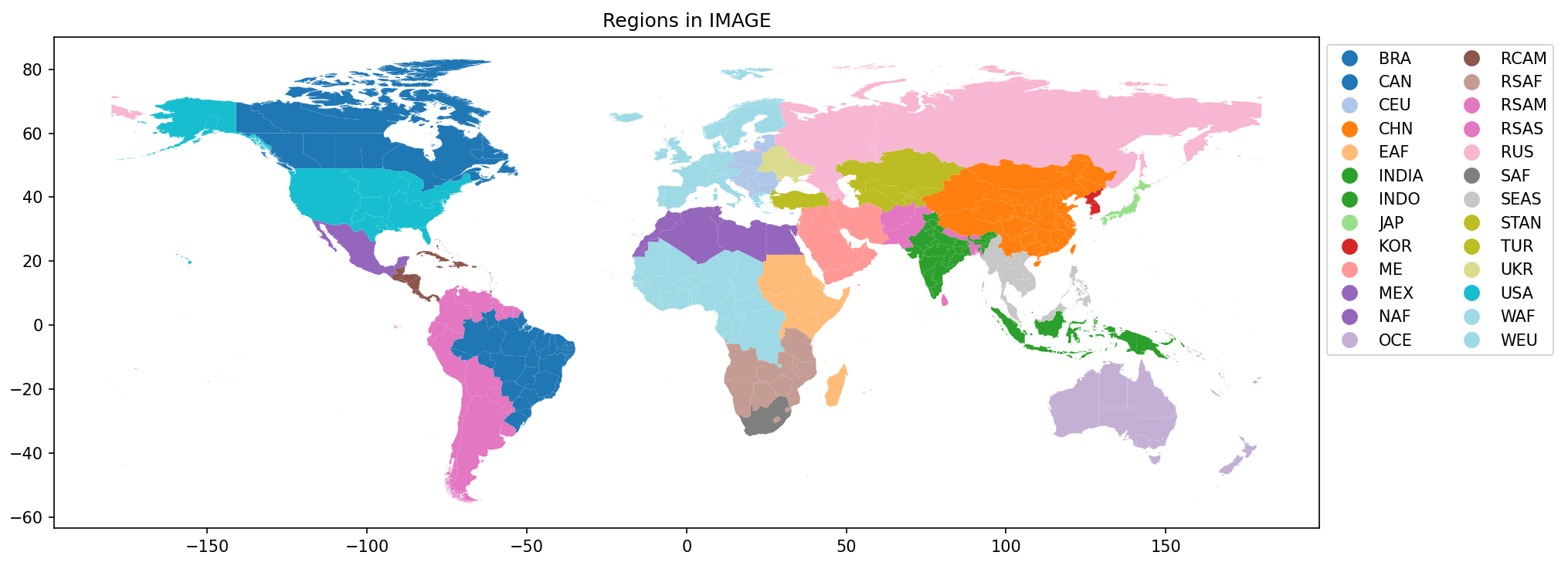
Map of REMIND regions

premise uses the following correspondence between ecoinvent locations and IAM regions. This mapping is performed by the constructive_geometries implementation in the wurst library.

ecoinvent location	REMIND region	IMAGE region
AE	MEA	ME
AL	NEU	CEU
AM	REF	RUS
AO	SSA	RSAF
APAC	OAS	SEAS
AR	LAM	RSAM
AT	EUR	WEU
AU	CAZ	OCE
AZ	REF	RUS
BA	NEU	CEU
BD	OAS	RSAS
BE	EUR	WEU
BG	EUR	CEU
BH	MEA	ME
BJ	SSA	WAF
BN	OAS	SEAS
BO	LAM	RSAM
BR	LAM	BRA
BR-AC	LAM	BRA
BR-AL	LAM	BRA
BR-AM	LAM	BRA
BR-AP	LAM	BRA
BR-BA	LAM	BRA
BR-CE	LAM	BRA
BR-DF	LAM	BRA
BR-ES	LAM	BRA
BR-GO	LAM	BRA
BR-MA	LAM	BRA
BR-MG	LAM	BRA
BR-Mid-western grid	LAM	BRA
BR-MS	LAM	BRA
BR-MT	LAM	BRA
BR-North-eastern grid	LAM	BRA
BR-Northern grid	LAM	BRA
BR-PA	LAM	BRA
BR-PB	LAM	BRA
BR-PE	LAM	BRA
BR-PI	LAM	BRA
BR-PR	LAM	BRA
BR-RJ	LAM	BRA
BR-RN	LAM	BRA
BR-RO	LAM	BRA
BR-RR	LAM	BRA
BR-RS	LAM	BRA
BR-SC	LAM	BRA
BR-SE	LAM	BRA
BR-South-eastern grid	LAM	BRA
BR-Southern grid	LAM	BRA
BR-SP	LAM	BRA
BR-TO	LAM	BRA
BW	SSA	RSAF
BY	REF	UKR
CA	CAZ	CAN
CA-AB	CAZ	CAN
CA-BC	CAZ	CAN
CA-MB	CAZ	CAN
Canada without Quebec	CAZ	CAN
CA-NB	CAZ	CAN
CA-NF	CAZ	CAN
CA-NS	CAZ	CAN
CA-NT	CAZ	CAN
CA-NU	CAZ	CAN
CA-ON	CAZ	CAN
CA-PE	CAZ	CAN
CA-QC	CAZ	CAN
CA-SK	CAZ	CAN
CA-YK	CAZ	CAN
CD	SSA	WAF
CENTREL	EUR	CEU
CG	SSA	WAF
CH	NEU	WEU
CI	SSA	WAF
CL	LAM	RSAM
CM	SSA	WAF
CN	CHA	CHN
CN-AH	CHA	CHN
CN-BJ	CHA	CHN
CN-CQ	CHA	CHN
CN-CSG	CHA	CHN
CN-FJ	CHA	CHN
CN-GD	CHA	CHN
CN-GS	CHA	CHN
CN-GX	CHA	CHN
CN-GZ	CHA	CHN
CN-HA	CHA	CHN
CN-HB	CHA	CHN
CN-HE	CHA	CHN
CN-HL	CHA	CHN
CN-HN	CHA	CHN
CN-HU	CHA	CHN
CN-JL	CHA	CHN
CN-JS	CHA	CHN
CN-JX	CHA	CHN
CN-LN	CHA	CHN
CN-NM	CHA	CHN
CN-NX	CHA	CHN
CN-QH	CHA	CHN
CN-SA	CHA	CHN
CN-SC	CHA	CHN
CN-SD	CHA	CHN
CN-SGCC	CHA	CHN
CN-SH	CHA	CHN
CN-SX	CHA	CHN
CN-TJ	CHA	CHN
CN-XJ	CHA	CHN
CN-XZ	CHA	CHN
CN-YN	CHA	CHN
CN-ZJ	CHA	CHN
CO	LAM	RSAM
CR	LAM	RCAM
CU	LAM	RCAM
CW	LAM	RCAM
CY	EUR	CEU
CZ	EUR	CEU
DE	EUR	WEU
DK	EUR	WEU
DO	LAM	RCAM
DZ	MEA	NAF
EC	LAM	RSAM
EE	EUR	CEU
EG	MEA	NAF
ENTSO-E	EUR	WEU
ER	SSA	EAF
ES	EUR	WEU
ET	SSA	EAF
Europe without Austria	EUR	WEU
Europe without Switzerland	EUR	WEU
Europe without Switzerland and Austria	EUR	WEU
Europe, without Russia and Turkey	EUR	WEU
FI	EUR	WEU
FR	EUR	WEU
GA	SSA	WAF
GB	EUR	WEU
GE	REF	RUS
GH	SSA	WAF
GI	EUR	WEU
GLO	World	World
GR	EUR	WEU
GT	LAM	RCAM
HK	CHA	CHN
HN	LAM	RCAM
HR	EUR	CEU
HT	LAM	RCAM
HU	EUR	CEU
IAI Area, Africa	SSA	RSAF
IAI Area, Asia, without China and GCC	OAS	SEAS
IAI Area, EU27 & EFTA	EUR	WEU
IAI Area, Gulf Cooperation Council	MEA	ME
IAI Area, North America	USA	USA
IAI Area, Russia & RER w/o EU27 & EFTA	REF	RUS
IAI Area, South America	LAM	RSAM
ID	OAS	INDO
IE	EUR	WEU
IL	MEA	ME
IN	IND	INDIA
IN-AP	IND	INDIA
IN-AR	IND	INDIA
IN-AS	IND	INDIA
IN-BR	IND	INDIA
IN-CT	IND	INDIA
IN-DL	IND	INDIA
IN-Eastern grid	IND	INDIA
IN-GA	IND	INDIA
IN-GJ	IND	INDIA
IN-HP	IND	INDIA
IN-HR	IND	INDIA
IN-JH	IND	INDIA
IN-JK	IND	INDIA
IN-KA	IND	INDIA
IN-KL	IND	INDIA
IN-MH	IND	INDIA
IN-ML	IND	INDIA
IN-MN	IND	INDIA
IN-MP	IND	INDIA
IN-NL	IND	INDIA
IN-North-eastern grid	IND	INDIA
IN-Northern grid	IND	INDIA
IN-OR	IND	INDIA
IN-PB	IND	INDIA
IN-PY	IND	INDIA
IN-RJ	IND	INDIA
IN-SK	IND	INDIA
IN-Southern grid	IND	INDIA
IN-TN	IND	INDIA
IN-TR	IND	INDIA
IN-UP	IND	INDIA
IN-UT	IND	INDIA
IN-WB	IND	INDIA
IN-Western grid	IND	INDIA
IQ	MEA	ME
IR	MEA	ME
IS	NEU	WEU
IT	EUR	WEU
JM	LAM	RCAM
JO	MEA	ME
JP	JPN	JAP
KE	SSA	EAF
KG	REF	STAN
KH	OAS	SEAS
KP	OAS	KOR
KR	OAS	KOR
KW	MEA	ME
KZ	REF	STAN
LB	MEA	ME
LK	OAS	RSAS
LT	EUR	CEU
LU	EUR	WEU
LV	EUR	CEU
LY	MEA	NAF
MA	MEA	NAF
MD	REF	UKR
ME	NEU	ME
MG	SSA	EAF
MK	NEU	CEU
MM	OAS	SEAS
MN	OAS	CHN
MT	EUR	WEU
MU	SSA	EAF
MX	LAM	MEX
MY	OAS	SEAS
MZ	SSA	RSAF
NA	SSA	RSAF
NE	SSA	WAF
NG	SSA	WAF
NI	LAM	RCAM
NL	EUR	WEU
NO	NEU	WEU
NORDEL	NEU	WEU
North America without Quebec	USA	USA
NP	OAS	RSAS
NZ	CAZ	OCE
OCE	CAZ	OCE
OM	MEA	ME
PA	LAM	RCAM
PE	LAM	RSAM
PG	OAS	INDO
PH	OAS	SEAS
PK	OAS	RSAS
PL	EUR	CEU
PT	EUR	WEU
PY	LAM	RSAM
QA	MEA	ME
RAF	SSA	RSAF
RAS	CHA	CHN
RER	EUR	WEU
RER w/o CH+DE	EUR	WEU
RER w/o DE+NL+RU	EUR	WEU
RER w/o RU	EUR	WEU
RLA	LAM	RSAM
RME	MEA	ME
RNA	USA	USA
RO	EUR	CEU
RoW	World	World
RS	NEU	CEU
RU	REF	RUS
RW	SSA	EAF
SA	MEA	ME
SAS	IND	INDIA
SD	MEA	EAF
SE	EUR	WEU
SG	OAS	SEAS
SI	EUR	CEU
SK	EUR	CEU
SN	SSA	WAF
SS	SSA	EAF
SV	LAM	RCAM
SY	MEA	ME
TG	SSA	WAF
TH	OAS	SEAS
TJ	REF	STAN
TM	REF	STAN
TN	MEA	NAF
TR	MEA	TUR
TT	LAM	RCAM
TW	CHA	CHN
TZ	SSA	RSAF
UA	REF	UKR
UCTE	EUR	WEU
UCTE without Germany	EUR	WEU
UN-OCEANIA	CAZ	OCE
UN-SEASIA	OAS	SEAS
US	USA	USA
US-ASCC	USA	USA
US-HICC	USA	USA
US-MRO	USA	USA
US-NPCC	USA	USA
US-PR	USA	USA
US-RFC	USA	USA
US-SERC	USA	USA
US-TRE	USA	USA
US-WECC	USA	USA
UY	LAM	RSAM
UZ	REF	STAN
VE	LAM	RSAM
VN	OAS	SEAS
WECC	USA	USA
WEU	EUR	WEU
XK	EUR	CEU
YE	MEA	ME
ZA	SSA	SAF
ZM	SSA	RSAF
ZW	SSA	RSAF

Regionalization

Several of the integration steps described above involve the regionalization of datasets. It is the case, for example, when introducing datasets representing a process for each of the IAM regions. In such case, the datasets are regionalized by selecting the most representative suppliers of inputs for each region. If a dataset in a specific IAM region requires tap water, for example, the regionalization process will select the most representative water suppliers in that region.

If more than one supplier is available, the regionalization process will allocated a supply share to each candidate supplier based on their respective production volume. If no adequate supplier is found for a given region, the regionalization process will select all the existing suppliers and allocate a supply share to each supplier based on their respective production volume.

Here is the decision tree followed:

Decision Tree for Processing Datasets

The process begins with a dataset that requires processing.

Decision: Is the Exchange in Cache?

• Yes

  • Use process_cached_exchange().

    • Retrieve cached data.

    • Update new_exchanges with cached data.

• No

  • Use process_uncached_exchange().

    • None

      • Print a warning and return.

    • One

      • Use handle_single_possible_dataset().

        • Use the single matched dataset.

        • Update new_exchanges with this dataset information.

    • Multiple

      • Use handle_multiple_possible_datasets().

        • Yes

          • Use the matched dataset location.

        • No

          • Use process_complex_matching_and_allocation().

            • IAM Region

              • Use handle_iam_region().

                • Match IAM region to ecoinvent locations.

                • Update new_exchanges with IAM region-specific data.

                • Cache the new entry.

            • Global (‘GLO’, ‘RoW’, ‘World’)

              • Use handle_global_and_row_scenarios().

                • Allocate inputs for global datasets.

                • Update new_exchanges with global data.

                • Cache the new entry.

            • Others

              • Perform GIS matching.

                • Determine intersecting locations with GIS.

                • Allocate inputs based on GIS matches.

                • Update new_exchanges with GIS-specific data.

                • Cache the new entry.

Final Steps

• If no match is found, use handle_default_option().

  • Integrate new exchanges into the dataset.

GAINS emission factors

Run

from premise import *
import brightway2 as bw

bw.projects.set_current("my_project)

ndb = NewDatabase(
    scenarios=[
            {"model":"remind", "pathway":"SSP2-Base", "year":2028}
        ],
    source_db="ecoinvent 3.7 cutoff",
    source_version="3.7.1",
    key='xxxxxxxxxxxxxxxxxxxxxxxxx'
)
ndb.update("emissions")

When using update(“emissions”), emission factors from the GAINS-EU and GAINS-IAM models are used to scale non-CO2 emissions in various datasets.

The emission factors are available under https://github.com/polca/premise/tree/master/premise/data/GAINS_emission_factors

Emission factors from GAINS-EU are applied to activities in European countries. Emission factors from GAINS-IAM are applied to activities in non-European countries, or to European activities if an emission facor from GAINS-EU has not been applied first.

Emission factors are specific to:

• an activity type,

• a year,

• a country (for GAINS-EU, otherwise a region),

• a fuel type,

• a technology type,

• and a scenario.

The mapping between GAINS and ecoinvent activities is available under the following file: https://github.com/polca/premise/blob/master/premise/data/GAINS_emission_factors/gains_ecoinvent_sectoral_mapping.yaml

The table below shows the mapping between ecoinvent and GAINS emission flows.

ecoinvent species	GAINS species
Sulfur dioxide	SO2
Sulfur oxides	SO2
Carbon monoxide, fossil	CO
Carbon monoxide, non-fossil	CO
Carbon monoxide, from soil or biomass stock	CO
Nitrogen oxides	NOx
Ammonia	NH3
NMVOC, non-methane volatile organic compounds, unspecified origin	VOC
VOC, volatile organic compounds, unspecified origin	VOC
Methane	CH4
Methane, fossil	CH4
Methane, non-fossil	CH4
Methane, from soil or biomass stock	CH4
Dinitrogen monoxide	N2O
Particulates, > 10 um	PM10
Particulates, > 2.5 um, and < 10um	PM25
Particulates, < 2.5 um	PM1

We consider emission factors in ecoinvent as representative of the current situation. Hence, we calculate a scaling factor from the GAINS emission factors for the year of the scenario relative to the year 2020. note that premise prevents scaling factors to be inferior to 1 if the year is inferior to 2020. Inversely, scaling factors cannot be superior to 1 if the year is superior to 2020.

Two GAINS-IAM scenarios are available:

• CLE: **C**urrent **LE**gislation scenario

• MFR: **M**aximum **F**easible **R**eduction scenario

By default, the CLE scenario is used. To use the MFR scenario:

ndb = NewDatabase(
    ...
    gains_scenario="MFR",
)

Finally, unlike GAINS-EU, GAINS-IAM uses IAM-like regions, not countries. The mapping between IAM regions and GAINS-IAM regions is available under the following file:

https://github.com/polca/premise/blob/master/premise/iam_variables_mapping/gains_regions_mapping.yaml

For questions related to GAINS modelling, please contact the respective GAINS team:

• GAINS-EU: https://gains.iiasa.ac.at/gains/EUN/index.login

• GAINS-IAM: https://gains.iiasa.ac.at/gains/IAM/index.login

Logs

premise generates a spreadsheet report detailing changes made to the database for each scenario. The report is saved in the current working directory and is automatically generated after database export.

The report lists the datasets added, updated and emptied. It also gives a number of indicators relating to efficiency, emissions, etc. for each scenario.

Finally, it also contains a “Validation” tab that lists datasets which potentially present erroneous values. These datasets are to be checked by the user.

This report can also be generated manually using the generate_change_report() method.